Visualising my journal writing
This week, I wanted to try an experiment by combining the efforts of my journal writing habits over the last four months with coding and data visualisation. So I thought the simplest thing I could do would be to create a visualisation of all the journal entries I’ve written this year.
Journal writing
Since the New Year, I’ve been getting up early in the morning to write. I try to write before I do anything else. I especially try to avoid reading anything else.
I have also occasionally written at other times in the day to see how it feels. But I feel writing first thing in the morning has been most effective. I start the day with a sense of small accomplishment and by doing this every day I have filled a few notebooks with entries of varying length. I will write about whatever comes into my head, be it dreams, the events of the day before, or some line of thought I want to pursue.
Whenever I write an entry, I note the date and place of the entry and I note the times I start and finish writing.
Recording data in a sheet
As I’ve done this, I’ve periodically recorded in a spreadsheet the dates and times of each entry, the start and end page numbers and journal type so that I can find the entry again quickly, and some notes on the subject and type of entry I’ve written.
This means I’ve got some data to play with on my relatively recent writing habit.
Here’s a sample:
| Date | Day | Start time | End time | Total time |
|---|---|---|---|---|
| 03/01/2016 | Sunday | 08:50 | ||
| 04/01/2016 | Monday | 06:00 | ||
| 05/01/2016 | Tuesday | 05:59 | ||
| 05/01/2016 | Tuesday | 06:30 | 07:20 | 00:50 |
| 06/01/2016 | Wednesday | 06:01 | ||
| 07/01/2016 | Thursday | 05:59 | 06:43 | 00:44 |
| 08/01/2016 | Friday | 06:05 | 06:50 | 00:45 |
| 08/01/2016 | Friday | 05:59 | 06:18 | 00:19 |
| 08/01/2016 | Friday | 17:00 | 17:27 | 00:27 |
| 09/01/2016 | Saturday | 08:15 | 09:33 | 01:18 |
| 10/01/2016 | Sunday | 07:25 | 07:58 | 00:33 |
| 11/01/2016 | Monday | 06:00 | 06:23 | 00:23 |
| 12/01/2016 | Tuesday | 06:03 | 06:38 | 00:35 |
| 13/01/2016 | Wednesday | 06:03 | 06:35 | 00:32 |
I didn’t always record an end time, particularly early on, so some of my data is incomplete.
Simple charts and graphs
I’ve been using Google Drive to keep the spreadsheet so that I can access and update it from numerous places with minimal hassle.
I had hoped to use the charts that come with Google Sheets to create some visualisations. However, I’ve found the prepackaged charts quite limited. I thought this might be the perfect excuse to explore D3, a JavaScript visualisation library.
Visualising differently
One of the limitations I found with Google Sheets is that I wanted to get some kind of view of the start and end times of each entry. But after some playing around with Google Sheets I couldn’t see how could one do this easily. The best I could manage was showing the total time against the date it was written.
It took me a while to find but I found that the kind of chart I wanted was called a “ranged bar graph”. I found this at a page from NC State University on bar graphs.
I found out this is also sometimes called a “floating bar” or “floating column” chart, as evidenced in a help page on Excel from Tech Republic.
I wondered what my journal entries data would look like when visualised as a series of dates across the x-axis and a series of times along the y-axis. I wondered, if I positioned each bar so that it started not at zero but at the time the entry started and ended at the end time, whether I could get a better sense of how my habit had shaped up over the last four or so months.
Learning how-to
To get familiar with what I’d need to do in D3, I started by reading Mike Bostock’s D3 bar chart tutorial.
I also found Scott Murray’s post on creating bar charts in D3 incredibly useful.
With D3, you mostly use SVG to create the visual elements one needs to represent the data. One quirk that I took from these tutorials is that SVG’s canvases position 0 in the top-left, whereas for most charts with positive axes, zero should be in the bottom-left. For this reason, one has to specify where from the top of the chart one wants the bar to begin. To set this, simply deduct the y-value from the height of the chart. If the height of the bar is then set to the value itself, it will reach the bottom of the graph.
Many of the tutorials I read used either a linear or an ordinal scale for the axes of the graphs. The linear scale is fine if you have a continuous range of possible values within which to specify your data. The ordinal scale allows for discrete and categories on an axis, for example a set of unrelated names or categories.
However, for my purposes I wanted a time scale on both axes, one showing dates, the other showing just the times (that is, the hour and minute elements of a date object).
Implementing the visualisation
First of all, I created an area for the chart as described in the tutorials mentioned above.
var margin = {top: 40, right: 40, bottom: 40, left: 40}
var width = 960
var height = 500

var svg = d3.select("body").append("svg")
    .attr("class", "chart")
    .attr("width", width)
    .attr("height", height)
  .append("g")
    .attr("transform", "translate(" + margin.left + ", " + margin.top + ")")
But before I could go further, I needed to make my data work. I copied the data directly from my Google Sheet into a text file and saved it as a .tsv file. Conveniently D3 has a method called d3.tsv, which works asynchronously – you can call a file with it, perform an accessor function on the data, and then pass it to a function where you can do things with it.
I put my data in data.tsv and came up with a simple function called cleanUpData:
d3.tsv("data.tsv", cleanUpData, function(error, data) {
    //...
})
The “clean up” function takes each object in my data and adds a few properties to it so that I could work with it more directly. The cleanUpData function called two other functions I wrote which did the date and time conversion.:
function cleanUpData (d) {
    d["date"] = convertUKDateToISO(d["Date"])
    d["start"] = convertTimeToJSDateTime(d["Start time"])
    d["end"] = convertTimeToJSDateTime(d["End time"])
    d["total"] = convertTimeToJSDateTime(d["Total time"])
    return d.date && d.start && d.end && d.total && d
}

function convertTimeToJSDateTime (t) {
    var minutes = /:(\d\d)$/.exec(t) || [ null, null ]
    var hours = /^(\d\d):/.exec(t) || [ null, null ]
    t = hours[1] && minutes[1] && new Date(0, 0, 0, hours[1], minutes[1])
    //console.log(t)
    return t
}

function convertUKDateToISO (d) {
    var d = d.split("/")
    d = d.length === 3 ? `${d[2]}-${d[1]}-${d[0]}` : null
    //console.log(d)
    return d
}
Within the callback for the file, I started specifying the domain of the data for each axis. For the x-axis, this was simply based on the dates of the first and last pieces of data in my file. This is because my data had already been chronologically sorted – though I will probably want to refactor the code to be more robust later.
var x = d3.time.scale()
    .domain([new Date(data[0].date), d3.time.day.offset(new Date(data[data.length - 1].date), 0)])
    .rangeRound([0, width - margin.left - margin.right])
For the y-axis, also a time scale, I asked D3 to find the earliest start time and the latest end time, using d3.min and d3.max respectively.
var y = d3.time.scale()
    .domain([d3.min(data, d => d.start), d3.max(data, d => d.end)])
    .range([height - margin.top - margin.bottom, 0])
Once, I’d done that I created and formatted the axes accordingly. For reasons of readability, I made the x-axis only show the names of each month, and the y-axis each hour of the day.
var xAxis = d3.svg.axis()
    .scale(x)
    .orient("bottom")
    .ticks(d3.time.days, 32)
    .tickFormat(d3.time.format("%B %Y"))
    .tickSize(5)
    .tickPadding(1)

var yAxis = d3.svg.axis()
    .scale(y)
    .orient("left")
    .ticks(d3.time.hours, 1)
    .tickFormat(d3.time.format("%H:%M"))
    .tickSize(10)
    .tickPadding(1)

svg.append("g")
    .attr("class", "x axis")
    .attr("transform", "translate(0, " + (height - margin.top - margin.bottom) + ")")
    .call(xAxis);

svg.append("g")
    .attr("class", "y axis")
    .call(yAxis)
  .append("text")
    .attr("transform", "rotate(-90)")
    .attr("y", 6)
    .attr("dy", ".71em")
    .style("text-anchor", "end")
    .text("Total time")
With all that in place, I “simply” added the bars to the chart. I say “simply” but it took a while to figure out how to do this.
svg.selectAll(".chart")
    .data(data)
  .enter().append("rect")
    .attr("class", "bar")
    .attr("x", function(d) { return x(new Date(d.date)); })
    .attr("y", function(d) { return y(d.end)})
    .attr("width", width / data.length)
    .attr("height", function(d) { return y(d.start) - y(d.end) })
One reason this took me so long is because the y(d.start) - y(d.end) seemed so counter-intuitive. If you want to find the difference between two numbers, you subtract the lower one from the higher one. My assumption was that d.end would be higher, being always later than d.start. However these values get passed through the y object which changes everything.
To test this, I actually passed two extreme cases to y to see what would happen. I passed it midnight (0.00) and the very last minute (23:59) of the very same day.
console.log("Extreme y values: ", y(new Date(0, 0, 0, 0, 0)), y(new Date(0, 0, 0, 23, 59)))
The former when put through y returned 420, the height of the chart, and the latter returned 0. So the end time would actually be lower than the start time in this case. Hence the ordering in the code above.
The result
I’m not yet entirely convinced by the results of all this work.
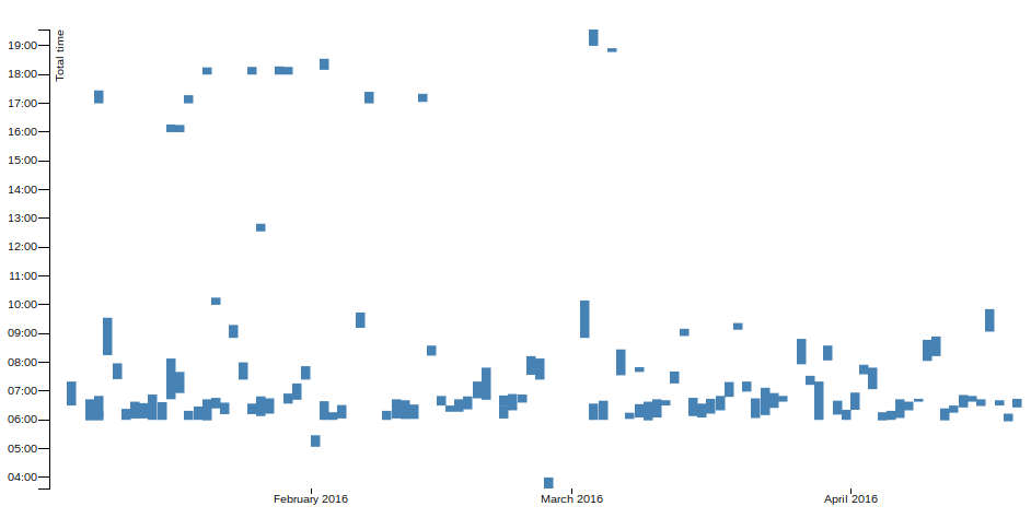
I’m glad I tried it as an exercise. But it’s my belief that visualisations should be able to show you something new, to reveal something about the data.
It may prove to be more useful to add some cosmetic tweaks to make the chart easier to read. I will need to spend more time with this to see what value I get from it.
My code
If you’re interested in seeing more on this and perhaps even playing around with the code and data yourself, I’ve made the full code available on a public repository called d3-testing. In addition to data.tsv which contains the data and index.html which contains the visualisation code, I have also added package.json and serve.json so the page can be served locally with Node.